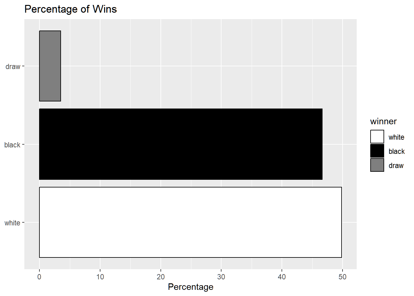
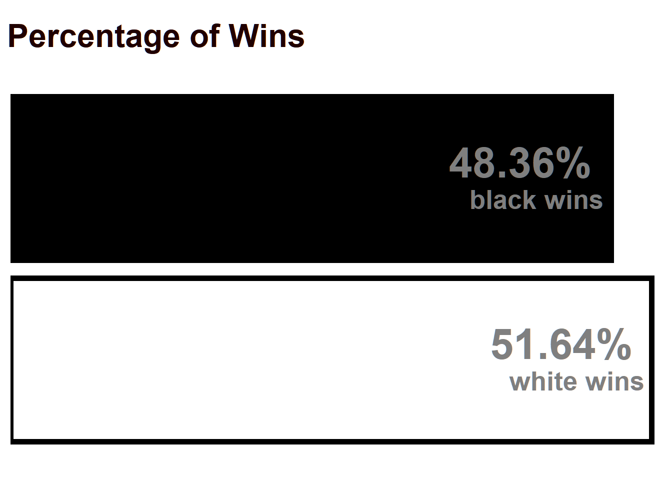
The main goal behind this is to check whether White has an advantage in Chess. We will use some of the concepts learnt in IPS to test and estimate this effect.
Warning in grid.Call(C_textBounds, as.graphicsAnnot(x$label), x$x, x$y, : font
family not found in Windows font database
Warning in grid.Call(C_textBounds, as.graphicsAnnot(x$label), x$x, x$y, : font
family not found in Windows font database
Warning in grid.Call(C_stringMetric, as.graphicsAnnot(x$label)): font family
not found in Windows font database
Warning in grid.Call(C_textBounds, as.graphicsAnnot(x$label), x$x, x$y, : font
family not found in Windows font database
Warning in grid.Call(C_textBounds, as.graphicsAnnot(x$label), x$x, x$y, : font
family not found in Windows font database
Warning in grid.Call(C_textBounds, as.graphicsAnnot(x$label), x$x, x$y, : font
family not found in Windows font database
Warning in grid.Call.graphics(C_text, as.graphicsAnnot(x$label), x$x, x$y, :
font family not found in Windows font database
Warning in grid.Call.graphics(C_text, as.graphicsAnnot(x$label), x$x, x$y, :
font family not found in Windows font database
Warning in grid.Call(C_textBounds, as.graphicsAnnot(x$label), x$x, x$y, : font
family not found in Windows font database
Warning in grid.Call(C_textBounds, as.graphicsAnnot(x$label), x$x, x$y, : font
family not found in Windows font database
Warning in grid.Call.graphics(C_text, as.graphicsAnnot(x$label), x$x, x$y, :
font family not found in Windows font database
Warning in grid.Call.graphics(C_text, as.graphicsAnnot(x$label), x$x, x$y, :
font family not found in Windows font database
Warning in grid.Call.graphics(C_text, as.graphicsAnnot(x$label), x$x, x$y, :
font family not found in Windows font database
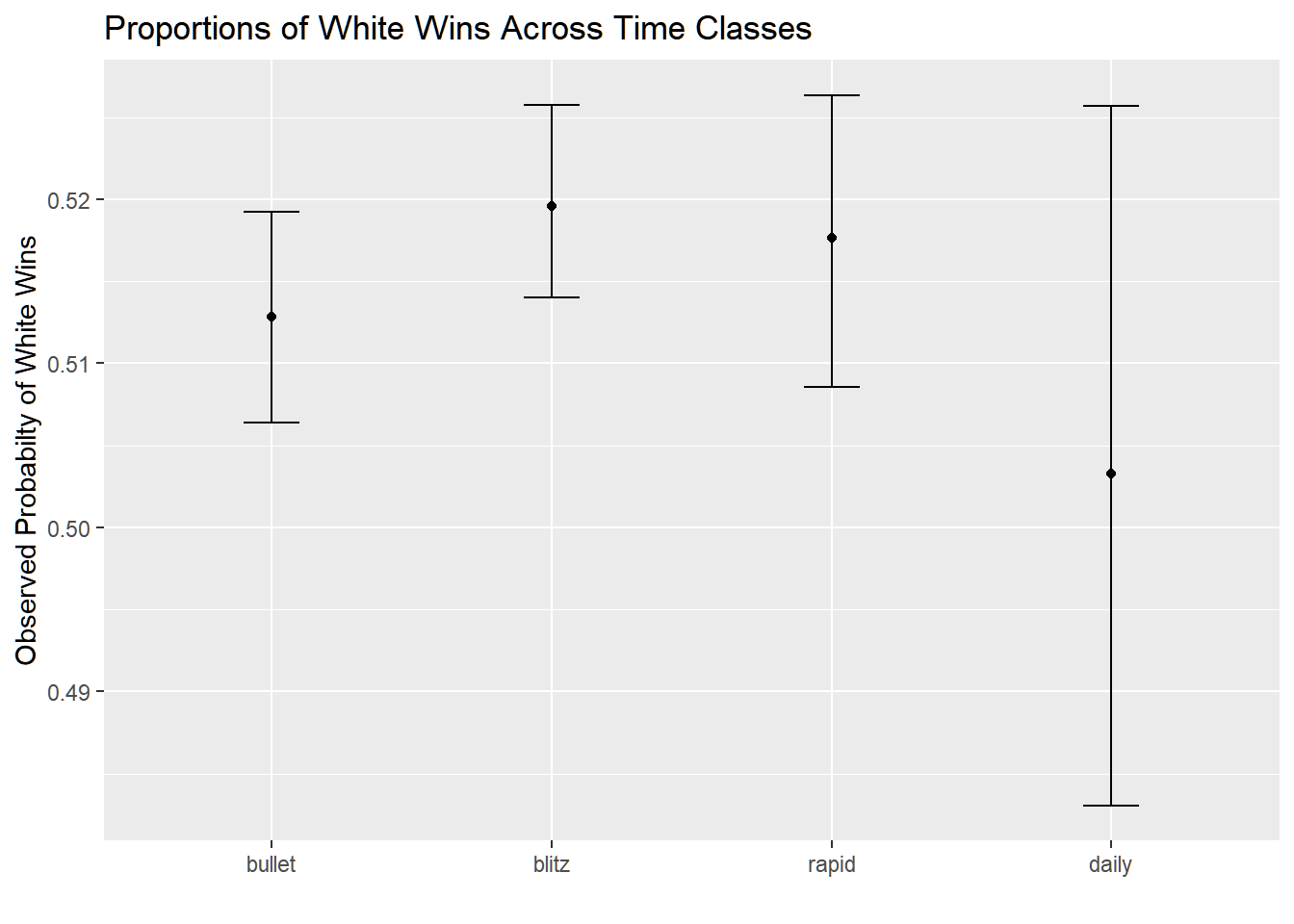
dat %>%mutate(white_win =ifelse(winner =="white", 1, 0)) %>%ggplot(aes(time_class, white_win)) +stat_summary(fun = mean, geom ="point") +stat_summary(fun.data = mean_cl_boot,geom ="errorbar",width =0.2) +theme(legend.position ="top") +labs(x ="", y ="Observed Probabilty of White Wins") +ggtitle("Proportions of White Wins Across Time Classes")
Methodology
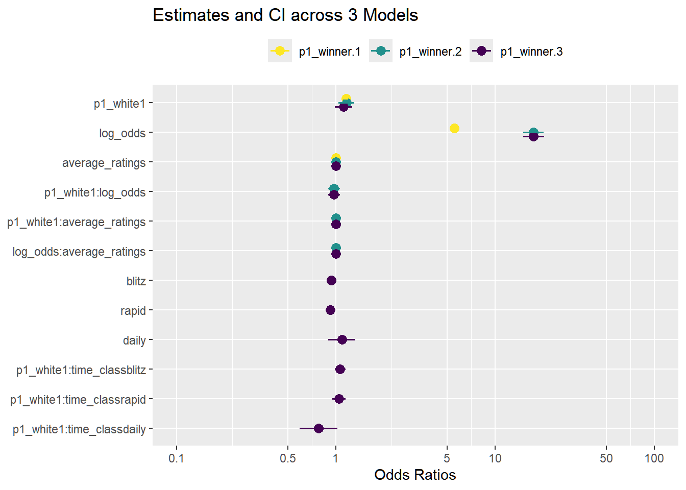
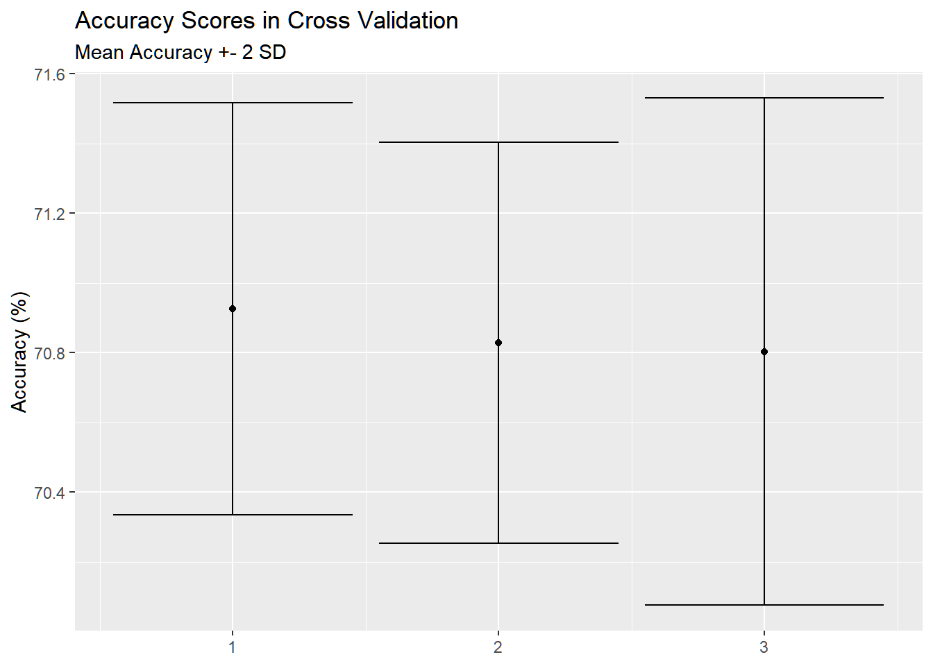
We will fit 3 models of varying complexity and select the one that results in the best predictions.
First, we need to change the data format to allow us to estimate the white advantage. Basically, we want to see how much does the probability of success of player changes if he plays white instead of black.
 p1_winner p1_white     log_odds          average_ratings   time_class
 0:31756   0:31813   Min.   :-10.724290   Min.   : 111.0   bullet:21727
 1:31724   1:31667   1st Qu.: -0.224502   1st Qu.: 983.4   blitz :27665
                     Median :  0.000000   Median :1252.0   rapid :12256
                     Mean   :  0.002473   Mean   :1248.6   daily : 1832
                     3rd Qu.:  0.224502   3rd Qu.:1521.5
                     Max.   : 11.789236   Max.   :2682.5
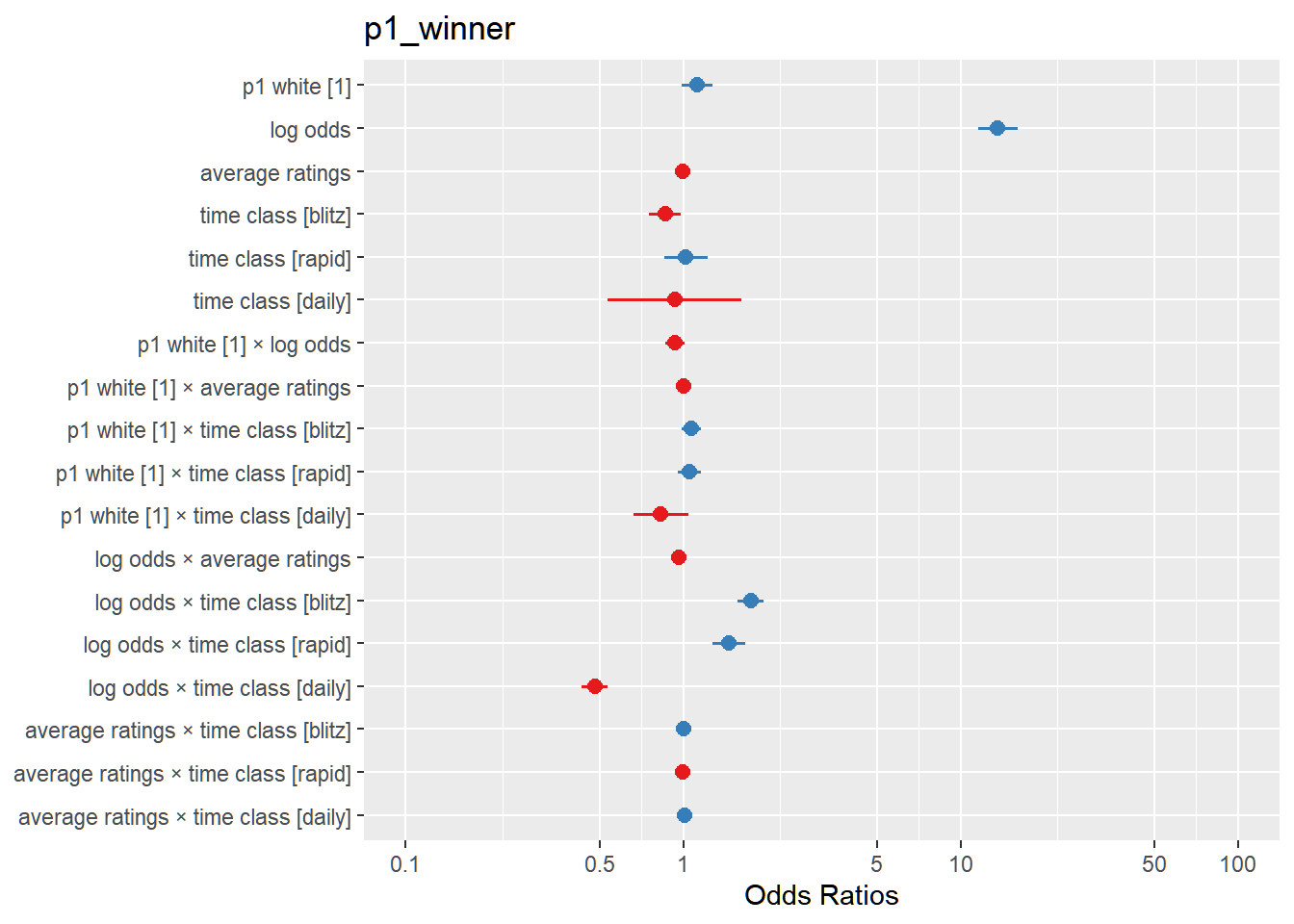
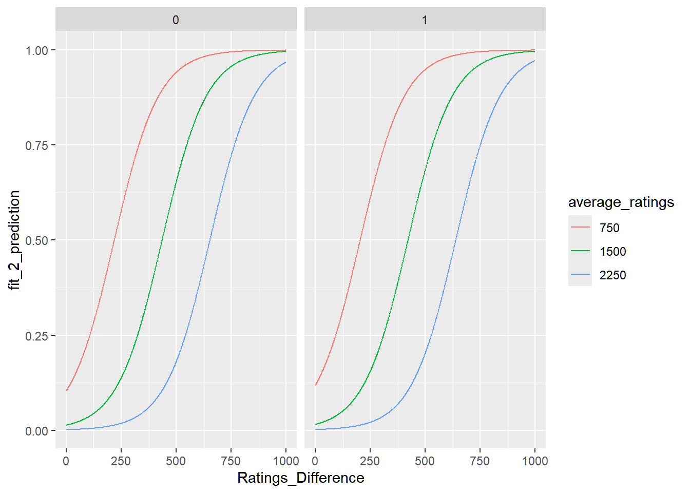
We will fit the model of increasing complexity on the above predictors. Interaction terms between p1_white and the other variables to see how the white advantage across skill, game, and player differences.
use K-Fold Cross Validation to determine the best model and analyse and visualize those results.
Models
Hi, we are pretty much only using logistic regression models.
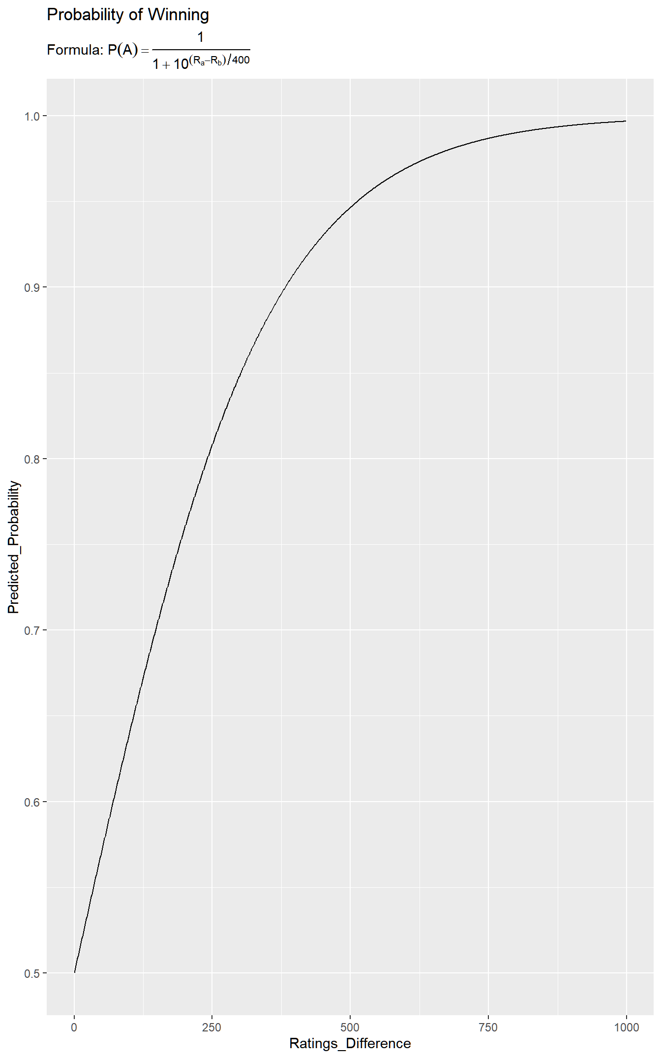
That means we are modeling the log odds of player 1 winning:
Warning in grid.Call(C_textBounds, as.graphicsAnnot(x$label), x$x, x$y, : font
family not found in Windows font database
Warning in grid.Call(C_textBounds, as.graphicsAnnot(x$label), x$x, x$y, : font
family not found in Windows font database
Warning in grid.Call(C_stringMetric, as.graphicsAnnot(x$label)): font family
not found in Windows font database
Warning in grid.Call(C_textBounds, as.graphicsAnnot(x$label), x$x, x$y, : font
family not found in Windows font database
Warning in grid.Call(C_textBounds, as.graphicsAnnot(x$label), x$x, x$y, : font
family not found in Windows font database
Warning in grid.Call(C_textBounds, as.graphicsAnnot(x$label), x$x, x$y, : font
family not found in Windows font database
Warning in grid.Call.graphics(C_text, as.graphicsAnnot(x$label), x$x, x$y, :
font family not found in Windows font database
Warning in grid.Call.graphics(C_text, as.graphicsAnnot(x$label), x$x, x$y, :
font family not found in Windows font database
Warning in grid.Call(C_textBounds, as.graphicsAnnot(x$label), x$x, x$y, : font
family not found in Windows font database
Warning in grid.Call(C_textBounds, as.graphicsAnnot(x$label), x$x, x$y, : font
family not found in Windows font database
Warning in grid.Call.graphics(C_text, as.graphicsAnnot(x$label), x$x, x$y, :
font family not found in Windows font database
Warning in grid.Call.graphics(C_text, as.graphicsAnnot(x$label), x$x, x$y, :
font family not found in Windows font database
Warning in grid.Call.graphics(C_text, as.graphicsAnnot(x$label), x$x, x$y, :
font family not found in Windows font database
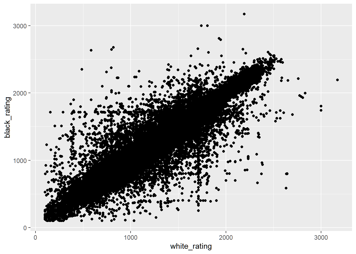
dat %>%ggplot(aes(white_rating, black_rating)) +geom_point()
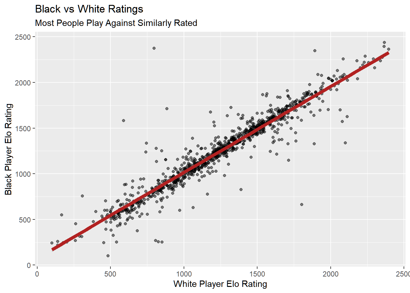
dat %>%sample_n(1000) %>%mutate(average_rating = (white_rating + black_rating) *0.5) %>%ggplot(aes(white_rating, black_rating)) +geom_point(alpha =0.5) +labs(x ="White Player Elo Rating",y ="Black Player Elo Rating",title ="Black vs White Ratings",subtitle ="Most People Play Against Similarly Rated" ) +geom_smooth(method ="lm", se =TRUE, color ="firebrick", linewidth =2)
`geom_smooth()` using formula = 'y ~ x'
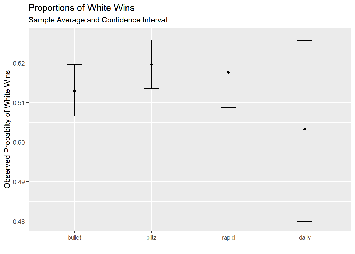
dat %>%mutate(white_win =ifelse(winner =="white", 1, 0)) %>%ggplot(aes(time_class, white_win)) +stat_summary(fun = mean, geom ="point") +stat_summary(fun.data = mean_cl_boot,geom ="errorbar",width =0.2) +theme(legend.position ="top") +labs(x ="", y ="Observed Probabilty of White Wins") +ggtitle("Proportions of White Wins", subtitle ="Sample Average and Confidence Interval ")
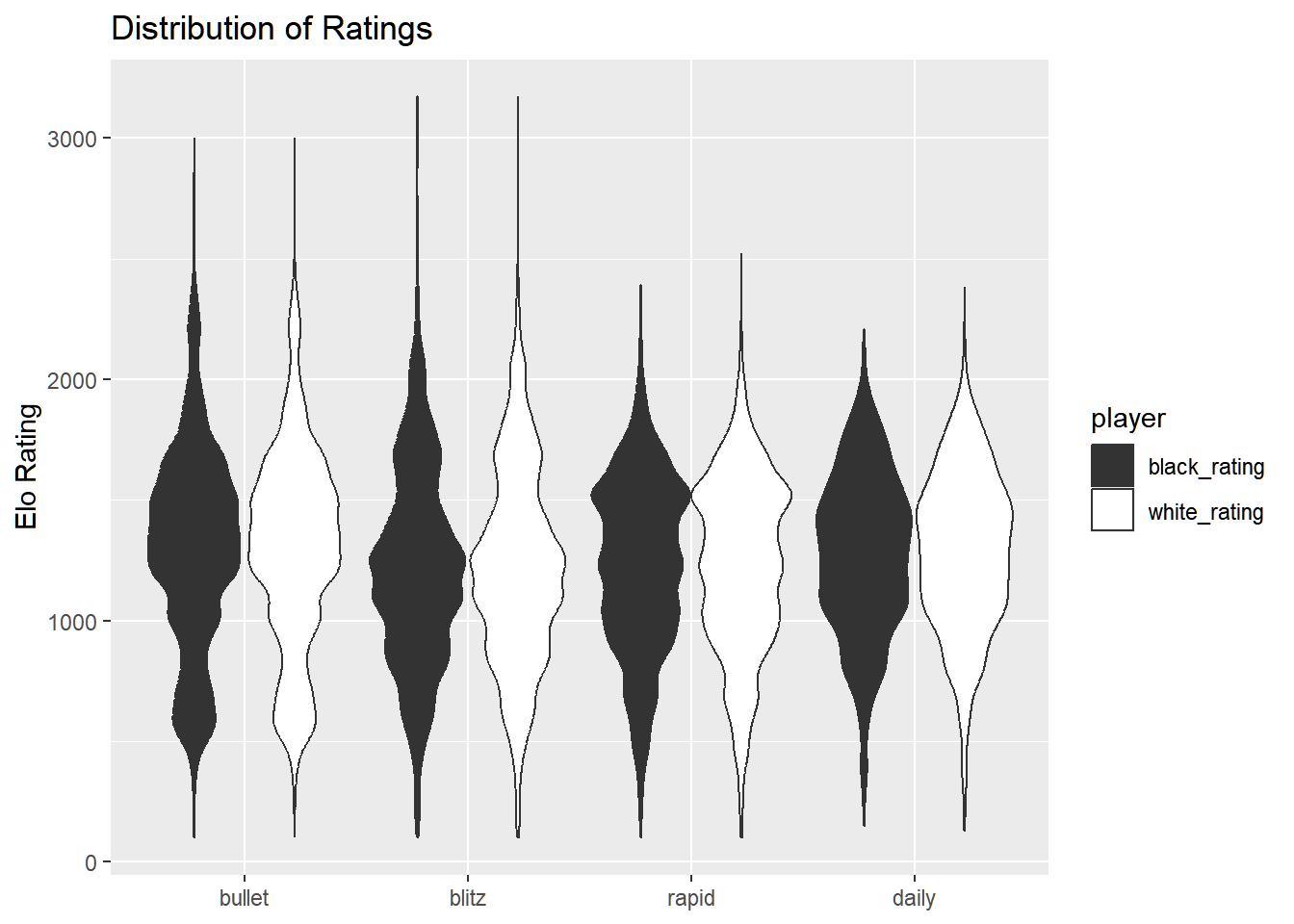
dat %>%pivot_longer(cols =ends_with("rating"),names_to ="player",values_to ="rating" ) %>%ggplot(aes(rating, time_class, fill = player)) +geom_violin() +scale_fill_manual(values =c("#333", "#fff")) +coord_flip() +labs(x ="Elo Rating", title ="Distribution of Ratings") +theme(axis.title.x =element_blank())
plot_models(mods) +scale_fill_discrete(name ="Model", labels =c("1", "2", "3"))+ggtitle("Estimates and CI across 3 Models") + viridis::scale_color_viridis(discrete = T) +theme(legend.position ="top", legend.title =element_blank())
Scale for colour is already present.
Adding another scale for colour, which will replace the existing scale.